The Baseline (Diagnosing the Naive Implementation)
Our first iteration of the code, fire_baseline.cpp, uses a standard approach for many beginner HPC
applications: the Asymmetric I/O Funnel.
Every 100 time steps, the simulation must write the current temperature of the grid to a binary file
for our Python visualizer. To do this, all MPI ranks call MPI_Gatherv to send their local chunks
of the grid over the network to Rank 0. Rank 0 stitches these chunks together in its memory and
performs a serial write to disk.
Let’s profile this baseline code with Linaro MAP on 16 processes using an 800x800 grid (as described in Compile and Profile Wildfire Simulation Proxy App) and look at the summary, “hot” MPI functions and MPI Call Statistics dialog (see MPI Call Statistics dialog):
Linaro MAP profiling summary
============================
Profiling time:      15 seconds (between MPI init and finalize)
Peak process memory: 74842112 B (~71.4 MiB)

Compute:              21.2%     (3.0s) |=|
MPI:                  78.2%    (11.0s) |=======|
I/O:                   0.6%     (0.1s) ||
  (based on time on the main thread)
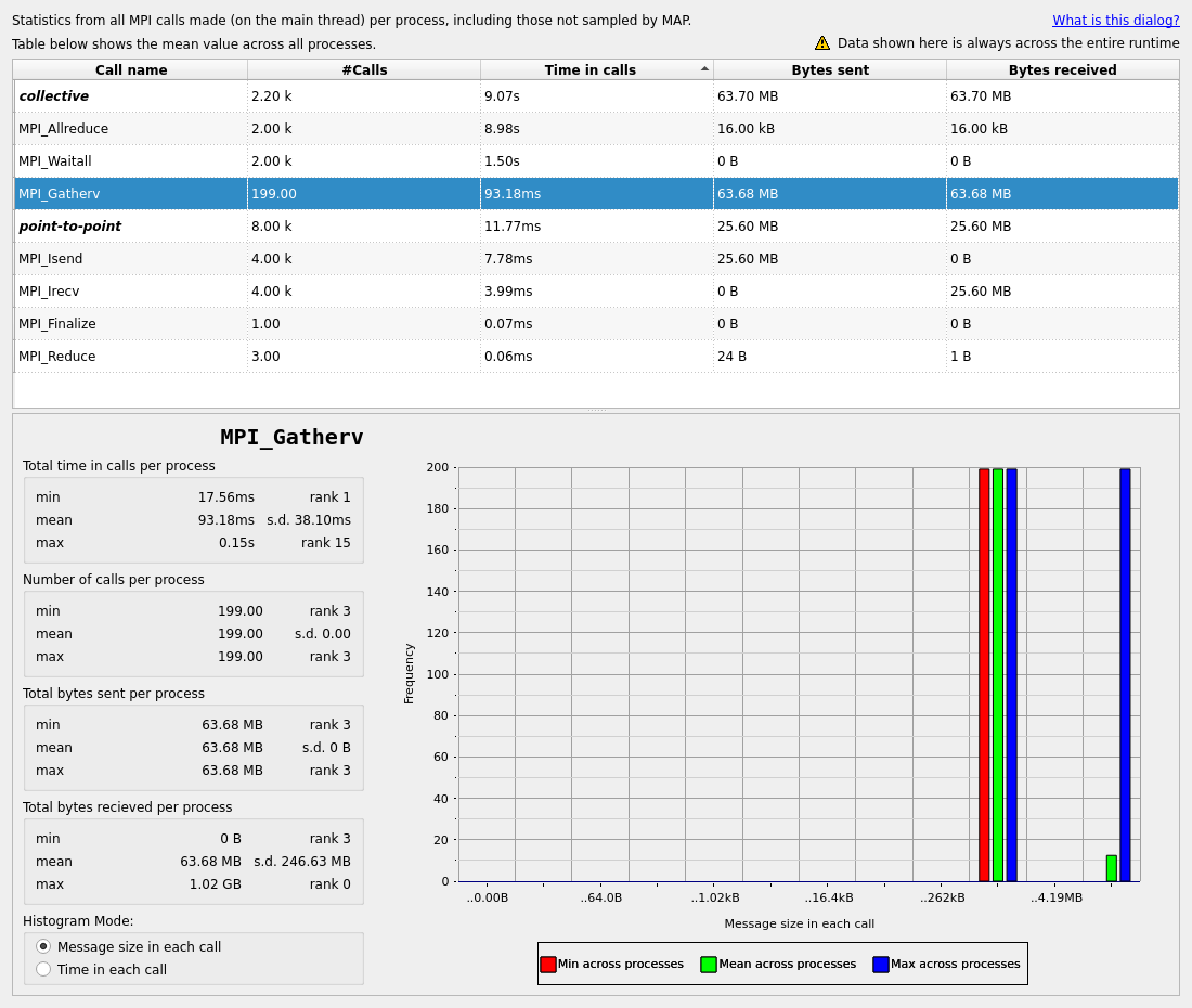
Fig. 25 The MPI Call Statistics of the baseline wildfire application run using an 800x800 grid for 2000 steps on 16 processes.

Fig. 26 The Parallel Stack View of the baseline wildfire application run using an 800x800 grid for 2000 steps on 16 processes.
66.0% of total wall time is spent waiting in MPI_Allreduce, 11.4% in MPI_Waitall and only 0.7% in MPI_Gatherv.
However we can see in the MPI Call Statistics window that Rank 0 receives 1.02 GB in the MPI_Gatherv call.
Let’s investigate the communication matrices to better understand the nature of the observed communication
bottlenecks and data transfers.
Diagnosis 1: The Asymmetric Funnel
Linaro MAP provides the Call, Volume and Time-wise MPI communication matrices. Let’s look at the Volume-wise matrix, which visualizes how much data is moving between specific ranks.
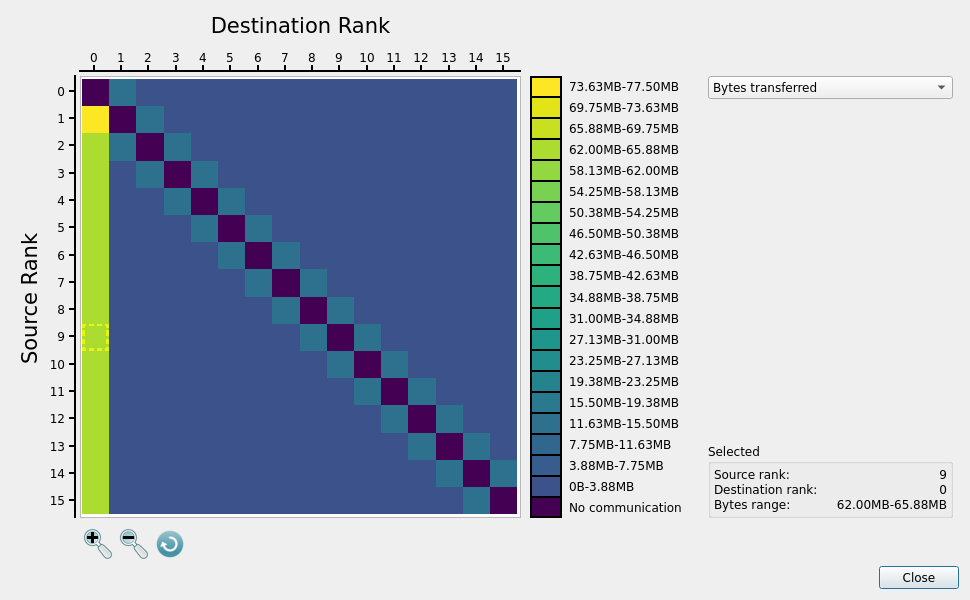
Fig. 27 Linaro MAP Volume-wise communication matrix for the baseline wildfire application run using an 800x800 grid for 2000 steps on 16 processes.
When looking at this matrix, you can see a solid lightly green left column (Rank 1 -> 0, Rank 2 -> 0, Rank 3 -> 0,
etc.). Along the two sub-diagonals, you will see faint blue squares representing our expected nearest-neighbor
halo exchanges, and some lower-volume traffic due to MPI_Allreduce calls.
Looking back at the MPI Call Statistics table, MPI_Gatherv accounts for 1.02 GB of the total data traffic.
Rank 0 is acting as a massive funnel. While this works on a tiny 16-core test, it is a
fatal architectural flaw. If we scaled this proxy app to 10,000 cores to run a high-resolution grid, Rank 0
would attempt to pull gigabytes if not terabytes of data into its RAM simultaneously, potentially resulting in an Out-Of-Memory
(OOM) crash.
Diagnosis 2: Load Imbalance (The Silent Straggler)
Next, we examine the Time-wise matrix, which shows where the simulation is spending its time.
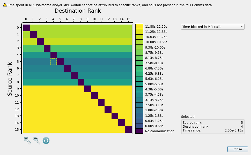
Fig. 28 Linaro MAP Time-wise communication matrix for the baseline wildfire application run using an 800x800 grid for 2000 steps on 16 processes.
Here we observe that ranks operating in the lower half of the grid (the Brush) show massive amounts of accumulated MPI time (solid yellow rows), while ranks in the top half (the Forest) rather reveal a spectrum of (mostly darker) colors.
This pattern reveals the heavy dynamic load imbalance present in our baseline implementation. Because we gave every processor exactly 50 rows, the work is heavily unbalanced:
The Blue to Green Ranks (Heavy Compute): Ranks processing the active forest fire are executing the heavy
std::exp()chemical kinetics loop many (initially 500) times per cell. Their CPUs are heavily utilized doing pure math, so they spend very little time in MPI calls.The Yellow Ranks (Light Compute): Mostly ranks processing the brush zip through their linear math almost instantly. They breeze into the halo exchange (
MPI_Waitall) and the global energy calculation (MPI_Allreduce), where they sit waiting. Some of the top rows also appear yellow (or lightly green) owing to the fact that fire has not reached respective ranks yet, or spent not enough time burning.
The fast ranks are forced to sit idle, trapped in collective barriers, waiting for the slow forest ranks to finish their math. Note that we see the spectrum of colors in the upper half due to the combination of the dynamic nature of the simulation, with fire spreading out as time goes (and burning most of the fuel in the center), and the fact that our communication matrix is static - reflecting total time spent in different ranks during all the 2000 steps.
On top of revealing the two bottlenecks cursing our baseline implementation, the communication matrices perfectly illustrate that high MPI time does not necessarily mean one has a slow network or is sending too much data. Instead it often indicates load-imbalance in the application.
To fix our proxy app, we must address both the I/O volume bottleneck and the CPU load imbalance.