Multi-Dimensional Array Viewer (MDA)
You can use the Multi-Dimensional Array Viewer (MDA) to view multi-dimensional arrays.
To open the Multi-Dimensional Array Viewer, right-click on a variable in the Source Code viewer, Locals tab, Current Line(s) tab or Evaluate window and select View Array (MDA). You can also open the MDA directly by selecting .
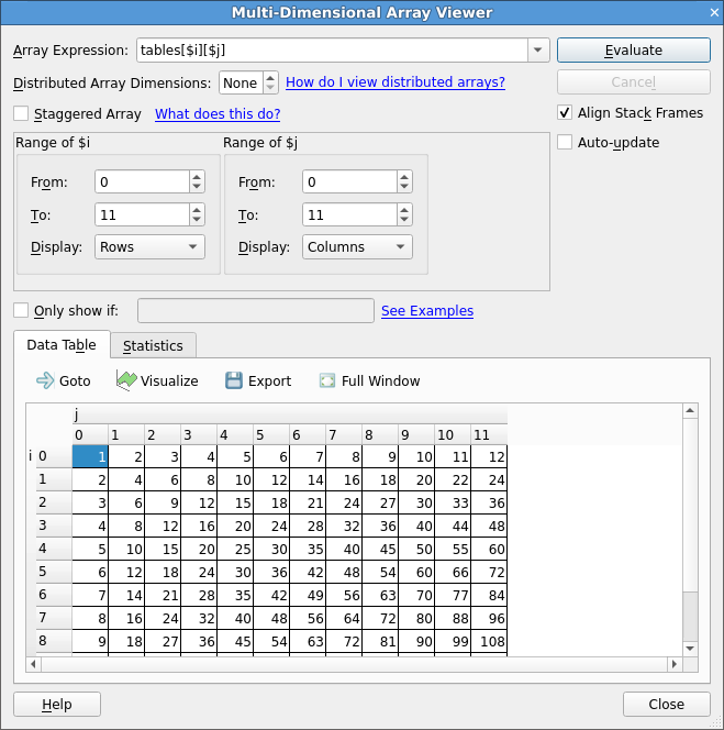
If you open the MDA by right-clicking on a variable, the Array Expression and other parameters will be automatically set based on the type of the variable. Click Evaluate to see the contents of the array in the Data Table.
Use Full Window to expand the table of values (and hide the settings at the top of the window). This enables you to make full use of your screen space. Click Full Window again to view the settings.
Array expression
The Array Expression is an expression containing a number of
subscript metavariables that are substituted with the subscripts of
the array. For example, the expression myArray($i, $j) has two
metavariables, $i and
$j. The metavariables are unrelated to the variables in your program.
The range of each metavariable is defined in the fields below the
expression, for example Range of $i. The Array Expression is
evaluated for each combination of
$i, $j, and so on. The results are shown in the Data Table. You
can control whether each metavariable is shown in the Data Table using
Rows or Columns.
By default, the ranges for these metavariables are integer constants entered using spin boxes. However, you can also specify these ranges as expressions in terms of program variables. These expressions are then evaluated in the debugger. To allow the entry of these expressions, select the Staggered Array checkbox. This converts all the range entry fields from spin boxes to line edits allowing the entry of free-form text.
The metavariables can be reordered by dragging and dropping them. For C/C++ expressions the major dimension is on the left and the minor dimension on the right. For Fortran expressions the major dimension is on the right and the minor dimension on the left. Distributed dimensions cannot be reordered, they must always be the most major dimensions.
Filter by value
You can configure the Data Table to only show elements that fit certain criteria, for example elements that are zero.
If the Only show if checkbox is selected, only elements that match the
boolean expression in the adjacent field are displayed in the Data Table.
For example,
$value == 0. The special metavariable $value in the expression is replaced
by the actual value of each element. The Data Table automatically hides
rows or columns in the table where no elements match the expression.
Any valid expression for the current language can be used here, including references to variables in scope and function calls. We recommend that you avoid functions with side effects as these will be evaluated many times.
Distributed arrays
A distributed array is an array that is distributed across one or more processes as local arrays.
The Multi-Dimensional Array Viewer can display certain types of distributed arrays, namely UPC shared arrays (for supported UPC implementations), and general arrays where the distributed dimensions are the most major, that is, the distributed dimensions change the most slowly, and are independent from the non-distributed dimensions.
UPC shared arrays are treated the same as local arrays. Right-click on the array variable and select View Array (MDA).
To view a non-UPC distributed array, create a process group that contains all the processes that the array is distributed over.
If the array is distributed over all processes in your job, select the All group when you right-click on the local array variable in the Source Code viewer, Locals tab, Current Line(s) tab or Evaluate window.
The Multi-Dimensional Array Viewer will open with the Array Expression already filled in.
Enter the number of Distributed Array Dimensions. A new subscript
metavariable (such as $p, $q) will be automatically added for each
distributed dimension.
Enter the ranges of the distributed dimensions so that the product is equal to the number of processes in the current process group, then click Evaluate.
Advanced: how arrays are laid out in the data table
The Data Table is two-dimensional, but the Multi-Dimensional Array Viewer can be used to view arrays with any number of dimensions, as the name implies. This section describes how multi-dimensional arrays are displayed in the two-dimensional table.
Each subscript metavariable (such as $i, $j, $p, $q) maps to a separate
dimension on a hypercube. Usually the number of metavariables is equal to the number of
dimensions in a given array, but this does not necessarily need to be the case. For
example myArray($i, $j) * $k introduces an extra dimension, $k, as well as the
two dimensions corresponding to the two dimensions of myArray.
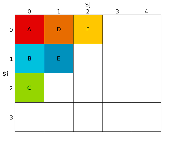
The figure below corresponds to the expression
myArray($i, $j) with $i = 0..3 and $j = 0..4.
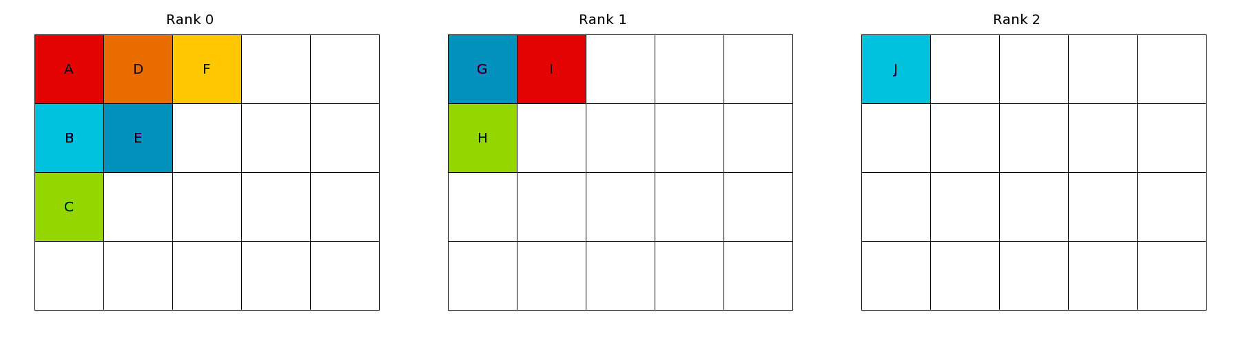
For example, imagine that myArray is part of a three-dimensional array distributed
across three processes. The figure below shows what the local arrays look like for each process.
This example shows the local array myArray($i, $j) with $i = 0..3 and $j = 0..4
on ranks 0-2.
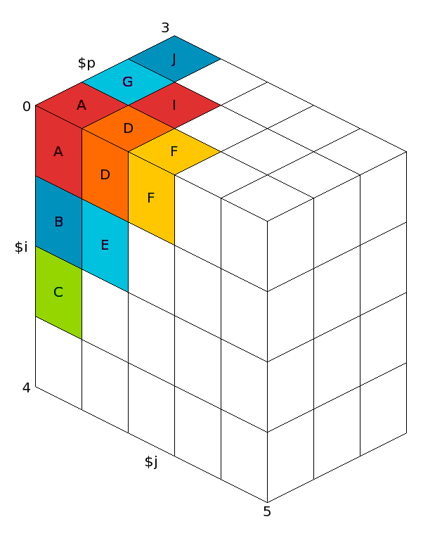
This figure shows a three-dimensional distributed array comprised of the local array
myArray($i, $j), with $i = 0..3, and $j = 0..4 on ranks 0-2, and with $p
the distributed dimension:
This cube is projected (just like 3D projection) onto the two dimensional Data Table. Dimensions marked Display as Rows are shown in rows, and dimensions marked Display as Columns are shown in columns, as you would expect.
More than one dimension may viewed as Rows, or more than one dimension viewed as Columns.
The dimension that changes fastest depends on the language your program
is written in. For C/C++ programs the leftmost metavariable (usually
$i for local arrays, or $p for distributed arrays) changes the most
slowly (just like with C array subscripts). The rightmost dimension
changes the most quickly. For Fortran programs the order is reversed,
that is the rightmost is most major, the leftmost most minor.
The figure below shows how the three-dimensional distributed array above is projected
onto the two-dimensional Data Table. This figure shows a three-dimensional
distributed array comprised of the local array myArray($i, $j) with $i = 0..3
and $j = 0..4 on ranks 0-2. It is projected onto the Data Table with $p (the
distributed dimension), $j displays as Columns, and $i displays as Rows:
Auto update
If you select the Auto update checkbox, the Data Table will automatically update as you switch between processes/threads and step through the code.
Compare elements across processes
When viewing an array in the Data Table, double-click an element or right-click an element and choose Compare Element Across Processes to open the Cross-Process Comparison View for the selected element.
See Cross-process and cross-thread comparison for more information.
Statistics tab
The Statistics tab displays information which might be of interest,
such as the range of the values in the table, and the number of special
numerical values, such as nan or inf.
Export
You can export the contents of the table to a file in the comma-separated values (CSV) or HDF5 format so that it can be plotted or analyzed in your favorite spreadsheet or mathematics program.
There are two CSV export options: List (one row per value), and Table (same layout as the on screen table).
Note
If you export a Fortran array in HDF5 format, the contents of the array are written in column major order. This is the order expected by most Fortran code, but the arrays will be transposed if read with the default settings by C-based HDF5 tools. Most HDF5 tools have an option to switch between row major and column major order.
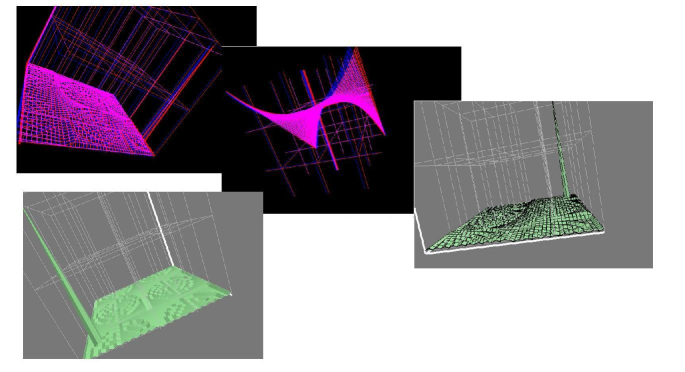
Visualization
If your system is OpenGL-capable then a 2-D slice of an array, or table of expressions, can be displayed as a surface in 3-D space using the Multi-Dimensional Array Viewer.
You can only plot one or two dimensions at a time. If your table has more than two dimensions the Visualize button will be disabled.
After filling the table of the MDA viewer with values, click Visualize to open a 3-D view of the surface.
To display surfaces from two or more different processes on the same plot, select another process in the main process group window then click Evaluate in the MDA viewer. When the values are ready, click Visualize again.
The surfaces displayed on the graph can be hidden and shown using the checkboxes on the right side of the window.
The graph can be moved and rotated using the mouse and a number of extra options are available from the window toolbar.
The mouse controls are:
Hold down the left button and drag to rotate the graph.
Hold down the right button to zoom. Drag forwards to zoom in, and backwards to zoom out.
Hold the middle button and drag to move the graph.
Note
Linaro DDT requires OpenGL to run. If your machine does not have hardware OpenGL support, software emulation libraries such as MesaGL are also supported.
Note
In some configurations OpenGL is known to crash. A workaround if the 3D visualization crashes is to set the environment variable LIBGL_ALWAYS_INDIRECT to 1. The precise configuration which triggers this problem is not known.
The toolbar and menu have options to configure lighting and other effects, including a function to save an image of the surface as it currently displays.