Overview

A short description of the main features of the OpenMP Regions view.

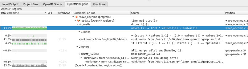
The OpenMP Regions view shows:

• The most time-consuming parallel region is in the update function at line 207. Clicking on this shows the region in the Source Code viewer.
• This region spends most of its time in the do_math function. Hovering on the line or clicking on the [–] symbol collapses the view down to show the figures for how much time.
• Of the lines of code inside do_math, the (sqtau * (values[i-1] ...) one takes longest with 13.7% of the total core hours across all cores used in the job.
• Calculating sqtau = tau * tau is the next most expensive line, taking 10.5% of the total core hours.
• Only 0.6% of the time in this region is spent on OpenMP overhead, such as starting/synchronizing threads.

From this you can see that the region is optimized for OpenMP usage, that is, it has very low overhead. If you want to improve performance you can look at the calculations on the lines highlighted in conjunction with the CPU instruction metrics, in order to answer the following questions:

• Is the current algorithm bound by computation speed or memory accesses? If the latter, you may be able to improve cache locality with a change to the data structure layout.
• Has the compiler generated optimal vectorized instructions for this routine? Small things can prevent the compiler doing this and you can look at the vectorization report for the routine to understand why.
• Is there another way to do this calculation more efficiently now that you know which parts of it are the most expensive to run?

See Metrics view for more information on CPU instruction metrics.

Click on any line of the OpenMP Regions view to jump to the Source Code viewer to show that line of code.

The percentage OpenMP synchronization time gives an idea as to how well your program is scaling to multiple cores and highlights the OpenMP regions that are causing the greatest overhead. Examples of things that cause OpenMP synchronization include:

• Poor load balancing, for example, some threads have more work to do or take longer to do it than others. The amount of synchronization time is the amount of time the fastest-finishing threads wait for the slowest before leaving the region. Modifying the OpenMP chunk size can help with this.
• Too many barriers. All time at an OpenMP barrier is counted as synchronization time. However, omp atomic does not appear as synchronization time. This is generally implemented as a locking modifier to CPU instructions. Overuse of the atomic operator shows up as large amounts of time spent in memory accesses and on lines immediately following an atomic pragma.
• Overly fine-grained parallelization. By default OpenMP synchronizes threads at the start and end of each parallel region. There is also some overhead involved in setting up each region. In general, the best performance is achieved when outer loops are parallelized rather than inner loops. This can also be alleviated by using the no_barrier OpenMP keyword if appropriate.

When parallelizing with OpenMP it is extremely important to achieve good single-core performance first. If a single CPU core is already bottlenecked on memory bandwidth, splitting the computations across additional cores rarely solves the problem.